
Completed in May 13, 2020 for Waubonsee Community College Honor Program, Business Statistics under the supervision of Dr. Collin Barnes
Abstract
This paper evaluates data from college basketball seasons in 2019 and 2018 to look for statistically significant results that can help predict the likelihood of tournament victories. Six different variables–offensive points per game, defensive points per game, offensive rebounds per game, free throw percentage, three-point percentage, and number of three-pointers allowed per game–are examined to determine if there is a better method in predicting tournament outcomes accurately than picking based on the higher seeded team. The first phase of testing uses analysis of variance (ANOVA) to determine round-by round if there are any difference in the means of teams that advance compared to teams that do not advance for all variables of study. The second series of testing uses multiple linear regression techniques to build a system of data models, where the different variables are the independent variables and the number of wins in the tournament is the dependent variable. The regression section uses brackets representing the model’s predictions to visualize the accuracy and precision of the model. The tests are evaluated statistically and critically throughout to discuss which discoveries of the investigation could be strong evidence or studied further. All data is compiled from the TeamRankings database website, and all tests were conducted through the data analysis tool kit in Microsoft Excel.
Keywords: College basketball, March Madness, ANOVA, multiple regression
March Madness Data Analysis Project
When the entire sports world is not shut down due to a deadly virus, March Madness is a staple of American sporting events. This 64 team, three-weekend single elimination tournament combines the thrill of constant action, high-pressure atmosphere, and millions of fans living and dying with their every matchup. However, the most popular tradition consists of the bracket challenge of successfully picking every winner of every game, known as the glorious perfect bracket. A perfect bracket is basically impossible; the number thrown around often when discussing the probability of a perfect bracket is 1 in 9.2 quintillion. That figure takes into account every possible combination of outcomes. Wilco (2020) estimates this number can reduce to about 1 in 120 billion for an average fan.
I have always considered myself an above average college basketball fan. Yet every year, my bracket is just as imperfect as the rest of the world. As I have grown closer to the game, I have realized I have several flaws in predicting games. Looking at March Madness from a statistical perspective, is there a way to compare and contrast teams in an unbiased way to make more educated picks and increase the likelihood of picking more winners in the tournament?
The traditional way of picking the most probable bracket is the chalk method: Picking the higher-seeded teams to win. The NCAA committee evaluates the seasons of every Division-I team, and then seeds them accordingly in the bracket, with 1-seed representing in theory the strongest teams while the 16-seeds represent in theory the weakest teams. This system of hierarchy probability wise has held up over time, as shown by the table from Jones (2020).
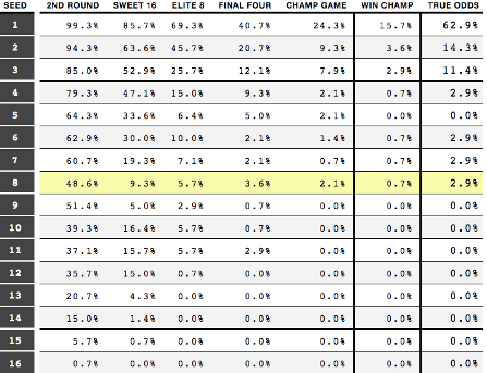
This data is the basis for the null hypothesis (Ho) for this project: Seeding is the most dependent way to project outcomes round-by-round. However, there are also observable holes in this method that align with common logic. The 8 vs. 9 matchups are essentially a coin flip. There is a 15% drop off between 4 and 5 seeds winning in the first round. And between the 10, 11, and 12 seeds, roughly one out of every three defeat a higher opponent. Moving out of the first round, as the teams become more evenly matched and higher quality, there is still a significant amount of opportunity for variation. As the tests are conducted, Seed will be the variable assumed to be best, and any other variables must show significant evidence they are equal or better to predicting likelihood of tournament victories.
These questions form the basis for the alternate hypothesis (Ha): Is there a variable or combination of variables that can better forecast tournament victories than the seed? The tournament is called March Madness for a reason—there is really no proven method for projecting tournament victories at a sustainable rate. Therefore, this paper will attempt to find possible relationships with between six different variables and number of tournament victories. Two methods from the Business Statistics curriculum will be used in this project: Analysis of Variance (ANOVA), and Multiple Linear Regression. The two most recent tournament data samples, 2019 and 2018, will be used for testing. The six variables are offensive points per game, defensive points per game, offensive rebounds per game, free throw percentage, three-point percentage, and number of three-pointers allowed per game. At this point, these variables must be defined further.
Definitions
Points scored per game (OPPG). Total points scored/ Number of games played. The goal of basketball on offense is to score more points than other team. Therefore, it is logical to assume the teams that score more points on average are more likely to score more points in the tournament, resulting in more victories. All six of these statistics are retrieved from the Team Rankings database. College basketball teams play 30-35 games over the course of the regular season. In statistics, 30 is a good number for a data set, as that is the point the data set takes the shape of a normal distribution. Therefore, by using the team averages per game, we assume an accurate point estimate that represents each team’s expected total output.
While the seasonal average gives a realistic outcome to expect, the randomness of the tournament means we cannot completely the offensive output per game to always be close to the point estimate, which is the mean value of all offensive outputs from the season. Every game becomes a random sample of one game from the season. This variable can also be affected by the overall caliber of defensive efficiency from their opponents throughout the season. In this project, one overall assumption is that strength of schedule is not important, as teams are judged purely by the merit of the raw data.
Points allowed per game (DPPG). Total points scored/Number of games played. On defensive, the goal of basketball is to stop other team from scoring. Like its counterpart OPPG, teams that allow fewer points play better defense, and are likely to win more games. “Defense wins championships” is a proverbial mantra in college basketball. Watching tournament games, this idea seems to hold true. The 2019 National Championship featured Virginia and Texas Tech, two of the most elite defenses in the country. The 2018 Final Four featured another defensive heavyweight in Michigan, in addition to Loyola-Chicago, who while seeded lower, showed a defensive caliber of play that carried them to the Final Four.
Defense is selected with higher expectations because unlike offense, it is less likely to vary. On offense, teams have off days, when the shots just are not falling. However, on defense, success is more related with effort, discipline, and teamwork than any specific skill. If a defensive minded team has a bad shooting game, they are more likely to make up for it by playing well on defense. In addition, every team plays better at home than on the road, but offense is more vulnerable to the crowd’s impact; in a college basketball game, the fans stand up and try to distract the opponent and motivate their players on defense. Therefore, “defense travels,” another common college basketball mantra, suggests location of game is not as significant for defensive minded teams. In a tournament where games are played at neutral locations, and the tilt of the crowd is difficult to statistically represent, measuring defense serves as a way to determine which teams are least impacted by the venue of the matchup.
Like OPPG, DPPG is open to sample variance, as one team can get hot for one game and score more than the defensive team can. UMBC beat the best defensive team in the tournament in 2018 (Virginia) because they made every shot and De’andre Hunter, Virginia’s best defender, was injured. There is not good way to statistically expect these wild outcomes. In addition, some defensive teams are just really bad on offense, so they can only play one way. This characteristic occurs much more frequently than a 16-seed beating a 1-seed.
Offensive rebounds per game (OREB). Total OREBs per game/Number of games played. The mindset behind testing OREB is simple: Teams that rebound missed shots at a higher rate increase likelihood of turning an unsuccessful possession into a successful one by scoring second-chance points, therefore adding a boost to offensive efficiency. Like defense, rebounding is less of a skill than it is a reflection of effort, so teams that rebound well express resiliency, and use height to an advantage.
As with all variables, the nature of the tournament means the number of offensive rebounds in a game can vary throughout the tournament. One specific way the offensive rebounding projection is prone to tournament randomness is in foul trouble. It is logical that the larger sample size from the regular season would account for how well the teams’ big men stayed out of foul trouble, but in the tournament, teams with rebounding disadvantages can attack inside to try and get the other team in foul trouble. In addition, securing an offensive rebound does not guarantee a second-chance conversion.
Free throw percentage (FT%). Total free throws made/Total free throws attempted. Free throws are a logical factor to use for March Madness because of the relative stability that can be expected. Because of how equally matched tournament games can be, a close game may come down to which team makes their free throws. Therefore, the team that is more dependable over the course of the regular season at the free throw line would be a more dependable team when converting free throws of high importance. Free throws are the only aspect of scoring the are not influenced by defense. While the atmosphere of the game (crowd, score, time remaining) can affect free throw shooting, for the purpose of the study it is assumed that these qualities cannot be measured.
Soppe (2020) provided support for free throws as a possible variable for projecting tournament victories, determining that in 2019 in the Round of 32, the team with the higher FT% advanced 13 out of 16 times. While this assertion is something to consider in the ANOVA tests, Soppe (2020) did not identify any other instances where FT% played a significant role in the two years of study. The conclusion reached was that for 2019, FT% was the variable that best represented offensive efficiency, so it cannot be assumed that these probabilities would hold true in other conditions.
3-point field goal percentage (3PT%). Total 3-pointers made/total 3-pointers attempted. The modern direction of basketball values three-point shooting at a high price, so developing a model evaluating the likelihood of tournament victories would be incomplete without testing potential significance of three-point shooting. Within the last decades, professional statisticians within the game of basketball have found convincing evidence for how three-point shooting is more analytically effective, causing a major shift across the entire sport. Part of this conclusion stems from the simple fact that three points is more than two, which gives lower seeded teams a better chance of keeping with the top teams because converting a higher rate outside shots can offset a talent gap. Additionally, teams that convert at high three-point rates can seize shifts in momentum and pull away from opponents faster, as seen with Villanova in 2018.
While the upside of 3PT% is substantial, there are a few drawbacks that could prevent the variable from showing statistical significance. The figure is prone to extensive variance because shooting varies game by game. Part of the reasoning for this phenomenon could be the varying effects of defense. In addition, three-point percentage does not take into account differences between quantity of threes attempted and quantity made. In other words, Team A may shoot 40% for 200 attempts for the season, while Team B shoots 36% for 300 attempts. Team A may have a better percentage, but Team B is more dependent on the three-point shot. By playing this style of basketball, Team B may sacrifice other important aspects of the game, compromising their well-rounded ability as a team.
Number of 3-pointers allowed per game (3PTD). Total three-pointers allowed/ # games played. This statistic responds to the addition 3PT%. Because we believe 3PT% may have a significant impact on determining outcomes of games, there should be an additional variable to account for how well teams prevent their opponent from taking advantage of the three-point line. Similar to DPPG, this number measures how well a team prevents their opponent from converting opportunities in the game. The difficulty in accounting for other defensive abilities can be a crucial flaw with this variable. For example, a team might have a low 3PTD because they are more vulnerable down in the post, so opponents spend less effort attempting threes. However, the approach that 3PTD is another way of measuring the impact of the three-point game is sufficient reasoning to test the variable in the study.
Methodology
ANOVA round-by-round comparison tests
Analysis of variance, or ANOVA, is a method of hypothesis testing comparing two or more treatment groups to determine if there is a significant difference between the different means. Microsoft Excel was used to compute the necessary ANOVA tables, determining the test statistic (F-distribution), strength of test statistic (p-value), and critical value for the rejection region. In order to reject the null hypothesis that there is no difference between the means, the value of the F-statistic had to exceed the critical value.
For this study, ANOVA was used to determine if there is a significant difference between the means for each of the seven variables round-by-round. There were four groupings of matchups for both 2019 and 2018: Round of 64 matchups, Round of 32 matchups, Sweet 16 matchups, and Elite 8 matchups. As the tests progressed with each round, the number of teams are narrowed down, so the decrease in degrees of freedom increases the critical value, meaning the test statistic must be higher moving through the tournament in order to prove a significant difference in the means. We use two treatments in each test: one with the variable of the teams who advanced in the round, and the other with the teams who lost in that round.
Decision Rules from round-by-round ANOVA tests of treatment variables (α =.05)
*2019 results are listed above 2018 tests for each variable
| Round of 64 | Round of 32 | Sweet 16 | Elite 8 | |
| SEED | Reject Ho | Reject Ho | Do not reject Ho | Do not reject Ho |
| Reject Ho | Do not reject Ho | Do not reject Ho | Do not reject Ho | |
| OPPG | Do not reject Ho | Do not reject Ho | Do not reject Ho | Do not reject Ho |
| Do not reject Ho | Do not reject Ho | Do not reject Ho | Do not reject Ho | |
| DPPG | Do not reject Ho | Do not reject Ho | Do not reject Ho | Do not reject Ho |
| Do not reject Ho | Do not reject Ho | Do not reject Ho | Do not reject Ho | |
| OREB | Reject Ho | Do not reject Ho | Do not reject Ho | Do not reject Ho |
| Do not reject Ho | Do not reject Ho | Do not reject Ho | Do not reject Ho | |
| FT% | Do not reject Ho | Reject Ho | Do not reject Ho | Do not reject Ho |
| Do not reject Ho | Do not reject Ho | Do not reject Ho | Do not reject Ho | |
| 3PT% | Do not reject Ho | Do not reject Ho | Do not reject Ho | Do not reject Ho |
| Do not reject Ho | Do not reject Ho | Do not reject Ho | Reject Ho | |
| 3PTD | Do not reject Ho | Do not reject Ho | Do not reject Ho | Do not reject Ho |
| Do not reject Ho | Do not reject Ho | Do not reject Ho | Do not reject Ho |
Discussion of ANOVA results. Of the 56 tests, the null hypothesis could only be rejected in six of the tests, when a significant difference between treatment means could be recorded. OPPG, DPPG, and 3PTD were never rejected, so there was no observable difference in the means for those variables between winning and losing teams. The other four however, showed indications they may be impactful, as at some point we rejected Ho and found evidence of a difference between means.
Starting with Seed, which we assume to be the best indicator of tournament success, the ANOVA test yielded very conclusive evidence for a difference of means in the Round of 64. Referencing the historic table of seed probability outcomes from Jones (2020), this outcome makes sense. The Round of 64 features the greatest mismatch between seeds of the six rounds, so it is safe to conclude that overall, Seed makes a difference in the first round.
Testing for Seed gets interesting moving into the Round of 32. 2019 showed strong evidence of a difference in means, but this may be unique to the top-heavy nature of the year. Considering the bracket, fifteen of the sixteen games were won by the higher seed, with 5-seed Auburn’s defeat of Kansas the lone underdog victory. However, in 2018, when Florida State, Kansas State, Loyola-Chicago, and Syracuse all advanced to the Sweet 16, there was almost no difference in the two means in the ANOVA test. Using only two sample years presents a flaw here as the natural variance from tournament to tournament found inconclusive results for the Round of 32.
Offensive rebounding looked to be the most promising of the other variables for early tournament matchups. In the Round of 64, the null hypothesis was rejected in 2019, and in 2018 the test statistic was 3.768, compared to the critical value of 3.996. While the null hypothesis cannot be rejected, the rather close F-value shows OREB made some semblance of a difference in 2018 for the Round of 64, just not enough to conclude at a .05 significance that there was a definite observable difference. After the Round of 64, there was little indication OREB had an observable difference among the treatment groups moving deeper into the tournament.
The statements in the definitions section may provide some explanation for why OREB impacted the tournament in the way shown by the ANOVA test, but the broad nature of OREB means further evidence is needed to verify if OREB truly is a major determinant of victory in the Round of 64. A natural method that can be applied for all any of these ANOVA tests is simply to test more years. If 2016 and 2017 show a similar pattern of offensive rebounding, then there would be strong evidence supporting offensive rebounding as a significant variable in predicting Round of 64 outcomes. Some more detailed examples could be evaluating categories such as second-chance points, or second chance conversion rates.
3PT% had a similar outcome as OREB, except the significant test occurred in the Elite 8. In 2018 the F-statistic exceeded the critical value, which is also notable because with a smaller sample size and degrees of freedom, the Elite 8 critical value was the highest of four rounds. In 2019, the F-statistic was considerably large, but not large enough for a rejection. In both years, three of the four teams that advanced to the final four were in the upper quartile of 3PT% in the field, while none of the teams that lost were among the 25% group of the field (Q1, Median, and Q3 regions are noted in the raw data totals in Appendices A and B). In addition, the only instance in either year where the team with the lower 3PT% lost was between Gonzaga and Texas Tech, which were separated by a mere 0.3% difference from their regular season average.
There can also be something to said for the round the difference in means occurred in. In the definitions section, one potential downside to 3PT% was how it may overvalue teams that are not as well-rounded. Considering the data analysis occurs in the Elite 8, it is valid to assume the teams are overall fairly complete, as they have already won three games in the tournament. Therefore, with all other variables unable to show a significant difference, teams that have an advantage in three-point shooting may have a sizable advantage. The data from 2019 and 2018 suggest there is considerable evidence that 3PT% is a key factor in determining which teams advance to the Final 4 from the Elite 8 matchups.
FT% is notable because it supports the principle Soppe (2020) proposed when defining FT%. The only time the ANOVA test yielded a test statistic above the critical value is in the Round of 32 in 2019. Therefore, the results of the ANOVA test confirm Soppe’s (2020) idea of FT% as an impactful variable in this specific instance. However, further application of FT% would need much stronger evidence, as no other ANOVA tests for FT% produced any F-values close to the critical value. Therefore, the rejection of the null hypothesis could very well be an isolated incident. Future years would definitely be the further area of study for this variable, as there are not many additional components to free throw shooting. One initial variable that was considered involved free throw shooting in the final four minutes of the game, but that data is not available anywhere yet.
The ANOVA tests helped accomplish one major task: determine which of the variables seemed influential in generating victories and which could not be confidently used to differentiate teams. The findings provide options for future investigation to determine if the significant differences between the treatment group means can be recognized as a dependable system of forecasting tournament victories. The three groups which had a rejection of the null hypothesis–OPPG, 3PT% and FT%–are good places to start any future studies. In addition, using actual tournament data instead of regular season estimations of performance using ANOVA testing could be the basis of another analysis. This format would look at what variables impacted actual games opposed to how these games could be predicted using average estimations of performance from the regular season population. At that point, each team can be evaluated by comparing their projected output from the regular season averages versus their actual output in the tournament. This method additionally could determine which variables are the most prone to variation in the tournament and would help answer some of the unknown aspects about the variables in the definitions section.
Regression Model for expected tournament wins
The second data analysis component of the study discusses multiple linear regression and creating a model of independent variables to determine how well they can predict the dependent variable. The Regression data analysis function in Microsoft Excel was used to calculate regression statistics. In this analysis, the focus will be on the r-squared term to assess what percentage of the variance can be explained by the independent variables within the model, and the p-value of the independent variables, which must be smaller than the significance of α =.05 in order to be included in the final models. Microsoft Excel’s regression package generates was used to generate coefficients for the multiple linear regression model, and then generates a predicted number of wins estimate from each team’s collection of data. The final value of interest was the residual amount, which can be determined by the number of actual wins less the number of predicted wins.
In the regression analysis, the dependent variable was the number of wins in the tournament, while the independent variables were Seed and the six test variables of the study. The initial regression testing started with a linear regression test for seed alone, and a multiple regression model for the other six variables, which will also be referred to as the Ha models because the variables of the alternate hypothesis were examined. Those variables were then assessed for significance, and variables with p < .05 remained in the model for further testing, while the others were removed. These variables were removed because they had insignificant effect on the r-squared value. Another model was then created using independent variables determined to be significant. The final model used the same variables determined to be of significance and added the seed variable to create the best model using all of the variables of study.
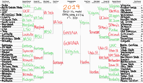
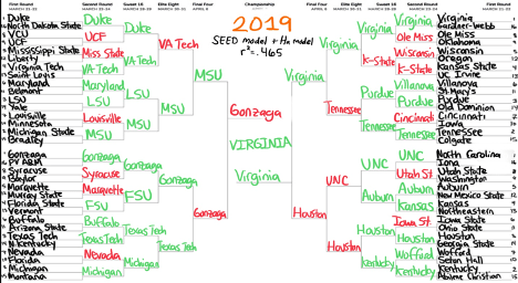
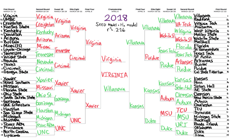
The visuals for the results of the predicted number of wins are demonstrated in bracket form. There are four models evaluated in this study (two for 2019 and two for 2018) which predict the outcomes of the matchups by advancing the team with the greater value for predicted number of wins in the specified model. Compared to the actual tournament results, the teams the model accurately predicted to win are in green, while teams that were inaccurately picked to win are in red.
For 2019, regression test for seed showed a moderate positive correlation, with an r-squared of .458, which can also be represented as declaring that 45.8% of the variance in outcomes can be determined by the seed. For the initial regression test for Ha, OPPG, DPPG, and FT% showed significant contribution to describing the variance, so OREB, 3PT% and 3PTD were no longer considered. When these variables were isolated, the r-squared term measured at .334. It should also be noted that at this point FT% started to become insignificant, as the p-value increased to above .05. The predicted wins from this regression model can be represented by the top bracket in Appendix C. At this point the two models were combined, which featured an r-square of .465. In this model, seed and DPPG were considered significant variables, and the model predicted the eventual national champion Virginia as the correctly with 3.21 predicted wins, defeating Gonzaga with 3.13 predicted wins.
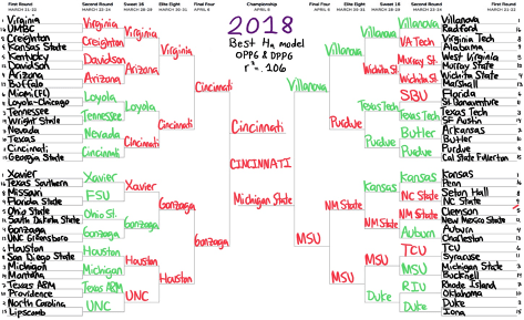
The process was the repeated for the 2018 data. In the initial Ha model, only OPPG and DPPG had significant p-values, and when isolated produced an r-squared value of .106, shown in the top bracket of Appendix D. The Seed model determined an r-squared of .294, which actually decreased to .216 by adding OPPG and DPPG, as neither variable tested significant when paired with Seed. Looking at the bottom bracket in Appendix D, the bracket is identical to what the bracket would look like for the predicted wins in the Seed model, as the higher team wins every game. Virginia was also predicted to win in 2018, which obviously did not go as planned.
Discussion of Regression Results. This process of testing may seem slightly counterintuitive, as essentially a prediction of the tournament results was created using the data from the tournament that already happened. The reasoning behind this manner of testing was to study how accurately the variables of interest projected accurate outcomes, and additionally to show what would have been the expected result had the tournament followed the laws of the model. The bottom brackets show the best model for the year which includes the Seed. For each year the top bracket features only the significant Ha variables and is included for reference to see the effects on the r-squared term when adding Seed to the model.
The method of combining regression models is not a true stepwise regression technique, so there are two approaches to interpret the strength of the model by the changes in r-squared. First looking at the 2019 data set, the changes could be viewed as either a 13.1% increase by adding Seed to the Ha model or a 0.7% increase to the Seed model by adding additional variables. In 2018, the changes could be interpreted as an 11% increase by adding the Seed to the Ha model or a 7.2% decrease to the Seed model.
Contrasting the two years from the regression statistics is not very difficult. While .465 is not an ideal r-squared value in the grand view of statistics, it is serviceable when looking for patterns in an event as chaotic as March Madness. With that said, looking at the bottom bracket of Appendix C, anyone who had that bracket would be in a respectable position. With a correct National Champion, another Final 4 team, and overall more green than red, this bracket could have been a lot worse. In addition, many of the games were toss ups in both the model and in the actual game, including Gonzaga vs. Texas Tech, Duke vs. Virginia Tech, Kentucky vs. Houston, and Tennessee vs. Purdue. Any of those four games going the other way (in favor of the model) could have made a momentous difference. The Ha is observably worse in real terms, and one potential flaw that may have been missing through the variable analysis was a strength of schedule component. New Mexico State had a chance to win at the buzzer against Auburn, but a deep run would have been a long shot. The models without seeds predicted far more upsets by 12-seeds and 13-seeds, as these positions are traditionally reserved for teams from weaker conferences, who have a good record and stats but do not play the caliber of opponents that most teams in the upper level of seeding do. The probability chart from Jones (2020) demonstrated how upsets by these lower-seeded teams do occur often, but the regression models do not offer any statistical insight as to which specific teams are likely to pull off a tournament upset.
On the other hand, the model .216 is less than serviceable, and the model shows there is was essentially no way to predict the craziness that occurred in the 2018 tournament. From the approach of this data study, these models were the best that could be made. However, the outlook is not all negative. Disregarding the mess in the upper-left portion of the bracket, the rest of the picks are not all that disastrous. In the model, North Carolina was .004 better than Michigan, so that game was a toss-up from the model’s perspective. The model additionally had both Villanova and Kansas in the Final 4, which is not unique as those the favorites to win their region, but 50% showing of correct Final 4 picks is admirable however it may be.
The bracket visuals were used to simplify the chart of predicted number of wins and put the data into context. One takeaway from the predicted values was how most teams had a value between -0.5 and 1.5 (For the record the only two teams that won with a negative prediction of wins were UMBC and Minnesota). Even the best teams from the model’s perspective could only be expected to win a maximum of two or three games. Initially a goal of this study was to determine if there was a suitable way to predict games deeper in the tournament. The regression analysis demonstrated how testing those matchups is extremely difficult. When 75% of the teams in the tournament win either one game or no games, separating the remaining 25% is a difficult task for even the best regression techniques.
CONLCLUSION
To put the discoveries of this investigation simply, there is significant evidence supporting “March Madness” as an appropriate name for the NCAA basketball tournament, as perfectly predicting the likelihood of tournament victories is difficult even using statistical techniques. However, while the results of the study show there are many factors that do not seem to impact the results of the tournament with large scale importance, the tests suggested certain variables may be significant at specific parts of the tournament. Offensive rebounding looked like a promising way to determine Round of 64 outcomes, while three-point percentage appeared to play a part in the Elite 8. Resolving the hypotheses statements for the study, despite small indications that the selected Ha variables can project the likelihood of tournament victories, picking higher seeds remains the best way to approximate tournament success.
Another component the study confirmed is that no two tournaments are identical. While 2018 featured a 16-seed beating a 1-seed and an 11-seed making the Final Four as the best offensive team in the country cut down the nets, 2019 featured fourteen of the higher seeds advancing to the Sweet 16 as the best defensive team in the country took home the championship. A two-year sample size is unlikely to accurately represent the storied chaos of the decades of the tournament’s existence, but as the most modern collection of data, it is a good starting point for experimentation.
This process has produced several ideas for future studies to test data for significance. The regression models showed a strong bias toward lower-seeded teams with good statistics, so there may be a strength of schedule component lacking in the model. Data from the actual tournament matchups could be substituted for the estimated value from the regular season average in the ANOVA section to test if there is a change in how any variables influence the outcomes of games. This study could also be further enhanced by testing additional years of data, specifically in areas where certain variables had a bigger impact. As long as the Coronavirus does not shut down sports forever, my studies into finding better ways to predict March Madness outcomes will continue in my quest for the perfect bracket, or more realistically applying methods learned in my statistics course to an event I am exceptionally interested in.
Appendix A: 2019 Data
| TEAM | #Wins | SEED | OPPG | DPPG | OREB | FT% | 3pt% | 3ptD |
| Virginia | 6 | 1 | 71.8 | 55.1 | 7.6 | 74.6% | 40.9% | 5.8 |
| Texas Tech | 5 | 3 | 73.1 | 59.3 | 8.0 | 72.8% | 36.8% | 6.3 |
| Michigan State | 4 | 2 | 78.8 | 65.5 | 9.6 | 75.0% | 38.4% | 7.3 |
| Auburn | 4 | 5 | 78.9 | 68.6 | 10.3 | 71.6% | 38.1% | 8.3 |
| Duke | 3 | 1 | 83.5 | 67.6 | 12.1 | 69.0% | 30.2% | 6.5 |
| Gonzaga | 3 | 1 | 88.8 | 65.1 | 8.5 | 76.7% | 36.5% | 6.6 |
| Kentucky | 3 | 2 | 76.7 | 65.4 | 10.2 | 74.0% | 36.4% | 7.8 |
| Purdue | 3 | 3 | 76.2 | 66.8 | 10.8 | 73.2% | 36.4% | 8.0 |
| North Carolina | 2 | 1 | 86.1 | 72.9 | 11.2 | 74.2% | 36.5% | 8.8 |
| Tennessee | 2 | 2 | 81.7 | 69.5 | 9.1 | 76.7% | 36.2% | 8.1 |
| Michigan | 2 | 2 | 70.4 | 58.6 | 6.6 | 69.8% | 35.0% | 4.7 |
| LSU | 2 | 3 | 81.4 | 73.0 | 12.4 | 75.4% | 32.3% | 7.8 |
| Houston | 2 | 3 | 75.6 | 61.2 | 10.9 | 70.2% | 35.9% | 6.3 |
| Florida State | 2 | 4 | 74.9 | 67.1 | 10.2 | 74.0% | 33.6% | 7.0 |
| Virginia Tech | 2 | 4 | 74.0 | 62.1 | 7.5 | 75.8% | 39.4% | 8.8 |
| Oregon | 2 | 12 | 70.5 | 62.9 | 8.4 | 71.9% | 34.3% | 7.1 |
| Kansas | 1 | 4 | 75.4 | 70.1 | 9.3 | 69.7% | 35.0% | 8.5 |
| Buffalo | 1 | 6 | 84.8 | 71.0 | 11.1 | 68.8% | 33.6% | 6.5 |
| Maryland | 1 | 6 | 71.3 | 65.1 | 9.4 | 74.8% | 35.3% | 7.4 |
| Villanova | 1 | 6 | 74.5 | 67.1 | 9.3 | 72.7% | 35.3% | 7.4 |
| Wofford | 1 | 7 | 81.2 | 67.5 | 9.5 | 70.5% | 41.6% | 7.2 |
| Baylor | 1 | 9 | 71.7 | 67.2 | 11.7 | 67.4% | 34.0% | 7.1 |
| UCF | 1 | 9 | 72.1 | 64.3 | 8.0 | 64.5% | 35.4% | 7.0 |
| Washington | 1 | 9 | 69.8 | 64.4 | 7.9 | 69.4% | 34.6% | 6.3 |
| Oklahoma | 1 | 9 | 71.2 | 68.2 | 7.6 | 69.1% | 34.2% | 8.4 |
| Minnesota | 1 | 10 | 70.8 | 69.2 | 9.4 | 67.9% | 32.1% | 6.7 |
| Florida | 1 | 10 | 68.3 | 63.6 | 9.1 | 71.8% | 33.5% | 6.4 |
| Iowa | 1 | 10 | 78.3 | 73.6 | 9.0 | 74.0% | 36.1% | 8.1 |
| Ohio State | 1 | 11 | 69.6 | 66.2 | 7.9 | 73.4% | 34.3% | 6.8 |
| Murray State | 1 | 12 | 81.6 | 68.4 | 9.9 | 74.1% | 34.4% | 6.1 |
| Liberty | 1 | 12 | 72.2 | 62.3 | 6.3 | 77.9% | 36.7% | 6.4 |
| UC Irvine | 1 | 13 | 72.5 | 63.6 | 9.9 | 70.0% | 36.0% | 6.2 |
| Kansas State | 0 | 4 | 65.8 | 59.2 | 8.0 | 66.4% | 33.6% | 6.8 |
| Mississippi State | 0 | 5 | 77.3 | 70.1 | 10.2 | 71.5% | 37.8% | 7.3 |
| Marquette | 0 | 5 | 77.7 | 69.1 | 8.0 | 75.9% | 39.3% | 6.8 |
| Wisconsin | 0 | 5 | 69.1 | 61.4 | 7.2 | 64.9% | 36.6% | 6.3 |
| Iowa State | 0 | 6 | 77.4 | 68.3 | 8.2 | 73.2% | 36.5% | 8.0 |
| Cincinnati | 0 | 7 | 71.7 | 62.2 | 10.9 | 70.4% | 35.0% | 8.0 |
| Louisville | 0 | 7 | 74.5 | 67.8 | 8.8 | 77.5% | 34.2% | 6.9 |
| Nevada | 0 | 7 | 80.7 | 66.7 | 8.0 | 70.8% | 35.1% | 7.8 |
| VCU | 0 | 8 | 71.4 | 61.6 | 9.5 | 69.8% | 30.7% | 5.1 |
| Utah State | 0 | 8 | 79.0 | 67.1 | 9.0 | 74.8% | 35.7% | 8.0 |
| Syracuse | 0 | 8 | 69.7 | 65.7 | 9.0 | 68.1% | 33.0% | 8.4 |
| Ole Miss | 0 | 8 | 75.4 | 70.4 | 8.1 | 78.3% | 35.9% | 7.3 |
| Seton Hall | 0 | 10 | 73.9 | 71.5 | 9.1 | 70.8% | 32.4% | 7.8 |
| Arizona State | 0 | 11 | 77.8 | 73.1 | 10.2 | 67.1% | 34.1% | 8.6 |
| St. Mary’s | 0 | 11 | 72.9 | 64.4 | 8.5 | 74.5% | 37.8% | 5.4 |
| Belmont | 0 | 11 | 86.9 | 74.7 | 7.6 | 73.6% | 37.1% | 7.7 |
| New Mexico St. | 0 | 12 | 77.7 | 64.8 | 11.9 | 67.3% | 35.1% | 7.0 |
| Saint Louis | 0 | 13 | 66.6 | 63.8 | 12.1 | 59.8% | 30.8% | 6.5 |
| Vermont | 0 | 13 | 72.4 | 62.8 | 7.8 | 75.3% | 35.3% | 7.2 |
| Northeastern | 0 | 13 | 76.1 | 70.3 | 6.1 | 75.1% | 38.8% | 6.8 |
| Old Dominion | 0 | 14 | 66.2 | 60.8 | 10.6 | 66.0% | 35.3% | 7.0 |
| N. Kentucky | 0 | 14 | 77.8 | 70.0 | 9.0 | 67.0% | 36.4% | 7.1 |
| Yale | 0 | 14 | 80.9 | 73.7 | 7.6 | 73.3% | 37.4% | 7.5 |
| Georgia State | 0 | 14 | 75.8 | 73.1 | 7.0 | 65.6% | 38.4% | 9.0 |
| Colgate | 0 | 15 | 75.5 | 70.1 | 8.3 | 74.3% | 39.1% | 8.0 |
| Abilene Christian | 0 | 15 | 71.7 | 64.9 | 8.1 | 72.3% | 38.3% | 5.7 |
| Bradley | 0 | 15 | 66.4 | 65.2 | 8.0 | 69.2% | 36.8% | 7.1 |
| Montana | 0 | 15 | 76.6 | 69.2 | 6.9 | 69.6% | 38.3% | 6.8 |
| FDU | 0 | 16 | 74.7 | 72.5 | 7.5 | 74.3% | 40.4% | 7.7 |
| Iona | 0 | 16 | 76.8 | 75.6 | 7.3 | 74.1% | 35.1% | 9.6 |
| Gardner-Webb | 0 | 16 | 75.8 | 73.4 | 5.9 | 71.6% | 37.7% | 9.3 |
| North Dakota St. | 0 | 16 | 72.3 | 73.7 | 5.6 | 76.5% | 36.8% | 7.6 |
| MEAN | 75.2 | 67.0 | 8.9 | 71.7% | 35.8% | 7.2 | ||
| MEDIAN | 75.2 | 67.1 | 8.9 | 72.1% | 35.9% | 7.2 | ||
| Q1 | 71.7 | 63.9 | 7.8 | 69.3% | 34.3% | 6.5 | ||
| Q3 | 77.8 | 70.1 | 10.1 | 74.5% | 37.3% | 8.0 | ||
| STANDARD DEV | 5.0 | 4.4 | 1.6 | 3.7% | 2.3% | 1.0 |
*Data retrieved from Team Rankings Database, through 03/18/2019
Appendix B: 2018 Data
| TEAM | #Wins | SEED | OPPG | DPPG | OREB | FT% | 3pt% | 3PTD |
| Villanova | 6 | 1 | 87.1 | 70.9 | 8.1 | 77.1% | 39.8% | 7.0 |
| Michigan | 5 | 3 | 73.6 | 63.5 | 7.7 | 65.7% | 36.3% | 5.6 |
| Kansas | 4 | 1 | 81.5 | 70.9 | 8.4 | 70.1% | 40.3% | 7.7 |
| Loyola-Chicago | 4 | 11 | 71.7 | 62.0 | 5.2 | 72.5% | 40.0% | 6.5 |
| Duke | 3 | 2 | 84.7 | 69.6 | 12.0 | 70.8% | 37.8% | 7.6 |
| Texas Tech | 3 | 3 | 75.2 | 64.7 | 9.5 | 70.1% | 36.6% | 6.9 |
| Kansas State | 3 | 9 | 72.4 | 67.9 | 7.0 | 74.2% | 34.4% | 7.1 |
| Florida State | 3 | 9 | 81.8 | 74.5 | 10.5 | 68.5% | 35.1% | 8.5 |
| Purdue | 2 | 2 | 81.1 | 65.6 | 7.2 | 74.3% | 42.0% | 6.9 |
| Gonzaga | 2 | 4 | 84.5 | 67.1 | 9.5 | 72.2% | 37.4% | 7.4 |
| Clemson | 2 | 5 | 73.3 | 65.8 | 7.7 | 75.7% | 36.6% | 7.6 |
| West Virginia | 2 | 5 | 79.6 | 69.0 | 12.2 | 76.6% | 35.3% | 7.5 |
| Kentucky | 2 | 5 | 76.7 | 70.3 | 10.8 | 69.7% | 36.1% | 7.6 |
| Texas A&M | 2 | 7 | 75.0 | 69.8 | 11.0 | 66.7% | 32.7% | 7.6 |
| Nevada | 2 | 7 | 83.1 | 72.9 | 8.4 | 74.7% | 39.8% | 7.5 |
| Syracuse | 2 | 11 | 67.5 | 64.5 | 10.2 | 74.0% | 32.1% | 7.9 |
| Xavier | 1 | 1 | 84.3 | 74.5 | 8.4 | 79.0% | 36.9% | 8.6 |
| Cincinnati | 1 | 2 | 74.5 | 57.1 | 11.5 | 68.7% | 35.7% | 6.4 |
| North Carolina | 1 | 2 | 82.0 | 73.1 | 12.1 | 74.1% | 36.4% | 9.7 |
| Michigan State | 1 | 3 | 81.0 | 64.8 | 10.0 | 75.1% | 41.3% | 7.3 |
| Tennessee | 1 | 3 | 74.2 | 66.4 | 10.0 | 75.6% | 38.4% | 6.4 |
| Auburn | 1 | 4 | 83.4 | 73.3 | 10.8 | 78.6% | 36.6% | 8.1 |
| Ohio State | 1 | 5 | 75.8 | 66.7 | 8.6 | 72.6% | 35.3% | 7.8 |
| Houston | 1 | 6 | 77.4 | 64.9 | 10.3 | 71.7% | 38.7% | 6.6 |
| Florida | 1 | 6 | 76.1 | 69.4 | 9.2 | 71.9% | 37.5% | 6.9 |
| Rhode Island | 1 | 7 | 76.2 | 67.9 | 9.8 | 70.7% | 35.0% | 5.2 |
| Seton Hall | 1 | 8 | 79.0 | 73.3 | 10.6 | 69.3% | 36.4% | 7.6 |
| Alabama | 1 | 9 | 72.4 | 70.0 | 8.9 | 67.2% | 32.5% | 6.9 |
| Butler | 1 | 10 | 79.1 | 72.8 | 7.4 | 77.1% | 35.6% | 7.8 |
| Buffalo | 1 | 13 | 84.7 | 76.5 | 10.2 | 69.6% | 37.2% | 6.8 |
| Marshall | 1 | 13 | 83.6 | 79.1 | 6.6 | 76.6% | 35.5% | 7.0 |
| UMBC | 1 | 16 | 72.5 | 71.0 | 7.7 | 65.0% | 38.2% | 8.3 |
| Virginia | 0 | 1 | 67.5 | 53.4 | 7.0 | 75.8% | 39.0% | 6.2 |
| Arizona | 0 | 4 | 80.9 | 71.2 | 9.0 | 76.1% | 37.7% | 7.2 |
| Wichita State | 0 | 4 | 83.0 | 71.3 | 10.2 | 73.8% | 38.5% | 8.5 |
| Miami (FL) | 0 | 6 | 74.2 | 68.0 | 8.3 | 66.3% | 36.3% | 6.7 |
| TCU | 0 | 6 | 83.0 | 75.9 | 9.6 | 70.8% | 40.0% | 8.1 |
| Arkansas | 0 | 7 | 81.1 | 75.5 | 8.7 | 67.8% | 40.0% | 8.5 |
| Missouri | 0 | 8 | 73.5 | 68.3 | 8.3 | 74.6% | 39.2% | 7.0 |
| Virginia Tech | 0 | 8 | 79.7 | 71.8 | 6.5 | 71.0% | 38.5% | 8.9 |
| Creighton | 0 | 8 | 84.0 | 75.1 | 6.2 | 74.9% | 37.6% | 7.9 |
| NC State | 0 | 9 | 81.2 | 74.5 | 10.2 | 70.1% | 37.2% | 6.0 |
| Texas | 0 | 10 | 71.7 | 68.2 | 9.4 | 66.8% | 31.5% | 6.8 |
| Providence | 0 | 10 | 73.7 | 72.7 | 8.8 | 70.3% | 33.3% | 6.9 |
| Oklahoma | 0 | 10 | 85.2 | 81.6 | 9.0 | 74.8% | 36.3% | 9.1 |
| San Diego State | 0 | 11 | 77.1 | 68.2 | 9.6 | 72.2% | 34.3% | 7.7 |
| St. Bonaventure | 0 | 11 | 77.9 | 71.0 | 9.0 | 75.4% | 39.8% | 7.7 |
| New Mexico State | 0 | 12 | 75.6 | 64.7 | 11.6 | 64.3% | 34.0% | 6.4 |
| Murray State | 0 | 12 | 77.4 | 66.0 | 9.0 | 72.8% | 37.4% | 6.3 |
| Davidson | 0 | 12 | 76.4 | 67.6 | 6.0 | 79.7% | 39.1% | 8.3 |
| South Dakota State | 0 | 12 | 83.4 | 75.6 | 7.5 | 76.4% | 39.2% | 8.1 |
| UNC Greensboro | 0 | 13 | 72.1 | 63.3 | 10.5 | 70.1% | 35.6% | 6.8 |
| Charleston | 0 | 13 | 75.2 | 69.8 | 7.3 | 76.8% | 36.3% | 7.2 |
| Wright State | 0 | 14 | 71.3 | 66.2 | 8.8 | 71.9% | 34.0% | 7.8 |
| SF Austin | 0 | 14 | 78.2 | 68.4 | 9.7 | 70.1% | 37.4% | 7.1 |
| Montana | 0 | 14 | 78.1 | 68.8 | 10.1 | 71.5% | 34.1% | 6.2 |
| Bucknell | 0 | 14 | 81.1 | 72.9 | 8.1 | 71.7% | 34.3% | 6.4 |
| Georgia State | 0 | 15 | 74.4 | 67.8 | 7.3 | 68.3% | 39.1% | 8.7 |
| Cal State Fullerton | 0 | 15 | 72.7 | 71.7 | 6.6 | 73.7% | 34.3% | 7.0 |
| Iona | 0 | 15 | 79.8 | 76.2 | 7.2 | 73.9% | 38.8% | 7.7 |
| Lipscomb | 0 | 15 | 80.9 | 78.5 | 8.9 | 72.5% | 33.0% | 7.4 |
| Radford | 0 | 16 | 66.9 | 64.9 | 9.2 | 73.3% | 35.1% | 6.9 |
| Penn | 0 | 16 | 75.7 | 69.6 | 7.4 | 66.3% | 34.7% | 5.8 |
| Texas Southern | 0 | 16 | 77.6 | 79.7 | 8.4 | 71.9% | 36.3% | 7.9 |
| MEAN | 77.7 | 69.8 | 8.9 | 72.2% | 36.7% | 7.3 | ||
| MEDIAN | 77.5 | 69.7 | 9.0 | 72.2% | 36.6% | 7.4 | ||
| Q1 | 74.2 | 66.5 | 7.7 | 70.1% | 35.1% | 6.8 | ||
| Q3 | 81.4 | 73.1 | 10.2 | 74.9% | 38.7% | 7.9 | ||
| STANDARD DEV | 4.7 | 5.0 | 1.6 | 3.6% | 2.3% | 0.9 |
*Data retrieved from TeamRankings Database, through 03/12/20
References
Jones, J. (2020). Bracketology: NCAA Tournament odds by Seed. Betfirm.
Soppe, K. (2020). How to get your Sweet 16 picks right when you fill out your bracket. ESPN.
https://www.espn.com/mens-college-basketball/story/_/id/28824072/how-get-your-
sweet-16-picks-right-fill-your-bracket
TeamRankings. https://www.teamrankings.com/ncb/stats/
Wilco, D. (2020). The absurd odds of a perfect NCAA bracket. NCAA.com.
https://www.ncaa.com/webview/news:basketball-men:bracketiq:2020-01-15:perfect-
ncaa-bracket-absurd-odds-march-madness-dream


Leave a comment